Daily insights for city builders, delivered every morning at 6 AM ET. I’m Brandon Donnelly — a Toronto-based real estate developer and founder of Globizen. I’ve been writing here since 2013.

Tag: chart

  • A comparative analysis of global cities

    Since 2005, LSE Cities (London School of Economics) has been collecting comparative data on how global cities perform in terms of key spatial, socioeconomic, and environmental indicators.

    This is their latest data matrix:

    To be clear, it is not a ranking of cities. It is intended to help us better understand how different cities around the world are performing.

    Depending on how you’re consuming this post, the text may be difficult to read. So here’s what each column represents, moving from left to right:

    • Current population in the administrative city (millions)
    • Current population in the urban agglomeration (millions)
    • Average hourly population growth of urban agglomeration 2015 to 2030 (people per hour)
    • Administrative city area (km2)
    • Average density of built-up administrative area (people/km2)
    • GDP per capita in urban area ($, PPP)
    • Percentage of country’s GDP produced by the metro region
    • Population under 20 (%)
    • Murder rate (homicides per 100,000 inhabitants)
    • Percentage of daily trips made by public transport
    • Percentage of daily trips made by walking & cycling
    • Car ownership rate (per 1,000 inhabitants)
    • CO2 emissions (tonnes per capita)

    If you’d prefer to download a full PDF of the chart, click here.

  • The Knight Frank Global Affordability Monitor 2019

    Here’s a chart from Knight Frank’s 2019 Global Affordability Monitor that I think you’ll find interesting:

    It compares real home price growth and real household income growth (after tax) over the last 5 years for 32 world cities. The bolded percentages represent the former and the non-bolded percentages represent the latter.

    Consider the variations here.

    Amsterdam saw a real home price change of 63.6%, but a household income change of only 4.4% (although the circle looks to be in the wrong spot if this number is correct).

    Moscow, on the other hand, saw flat home prices (0.1%) and a 22.7% increase in household income.

    Though San Francisco is the star in terms of income growth.

    Sao Paulo, unfortunately, saw a dramatic decline in both home prices and incomes. It’s in the bottom left corner.

    When I look at this chart, I don’t see a strong correlation between household incomes and home prices. And the proportions of the chart tell you that the y-axis is moving more than the x-axis.

    But if the top number exceeds the bottom number, then you could come to the conclusion that housing affordability has gotten worse over the last 5 years.

  • Where Canada’s immigrants have come from

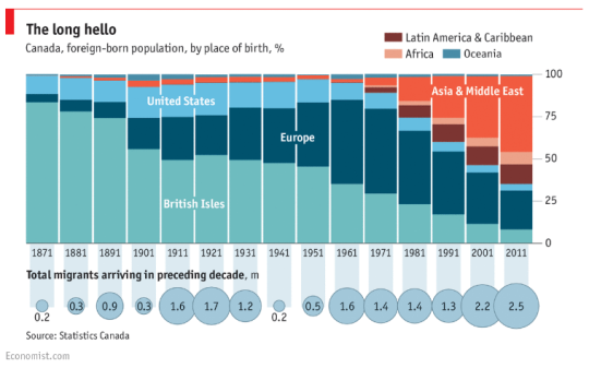
    Earlier today The Economist published the below chart showing where Canada’s immigrants have come from (place of birth) between 1871 and 2011. So basically from Confederation (1867) to today – almost.

    It’s a great chart. It really shows our evolution.

    Perhaps the most meaningful date to point out is 1962. That is the year Canada introduced new immigration regulations which effectively privileged skill and talent over race and national origin when it came to deciding who would be allowed to enter the country. 

    Look at the impact that had.

  • The urban wealth pendulum

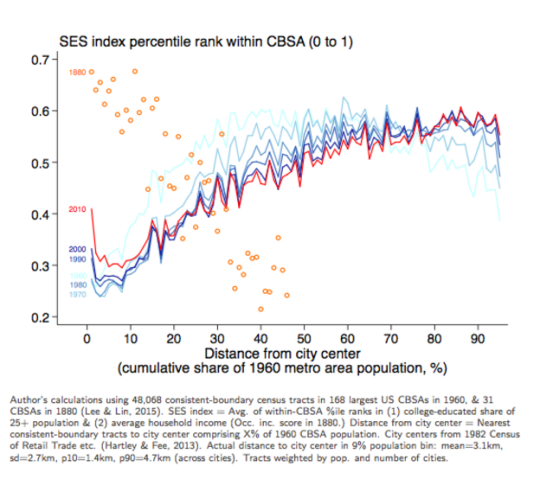
    Jeffrey Lin, who is an economist at the Federal Reserve Bank of Philadelphia, recently published the following chart:

    image

    I found it in this Washington Post article. And it’s packed full of fascinating information.

    The chart compares the socioeconomic status in US cities (y-axis) against “distance from city center” (x-axis) in 1880 and then in recent years (1960 to 2010 census data). The orange circles represent the 1880 data and the red and blue lines represent the recent census data.

    What this chart and research tells us is that in 1880, rich people overwhelmingly lived in the center of cities. And as you moved further away from the city center, socioeconomic status fell off pretty precipitously. This makes sense given that, at the time, it was hard to get around and travel long distances.

    However, in the post-war years, the exact opposite became true. We began driving and wealth decentralized. This should surprise no one. 

    But what’s interesting is how this appears to be reversing. In 2010 (the red line), there’s a sharp increase in socioeconomic status for people living basically right in the center of cities. And for the 30 – 60 km range, there has been a decrease in socioeconomic status essentially from the 1960s onwards. 

    The important takeaway here – which is spelled out in the Washington Post article – is that the neighborhoods which appear to be in high demand today are also in very short supply:

    “We have 80 years of essentially zero production of neighborhoods with these qualities,” Grant says. “We’ve spent the last 80 years building car-oriented suburbs. Then when the elites decide they want to go back into the city, there’s not enough city to go around.”

    This is one reason why supply matters.

  • This U.S. housing boom is different

    Just a few days ago, The Federal Reserve Bank of San Francisco published an interesting research study where they argue that this U.S. housing boom is different than that of the early 2000s.

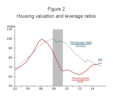
    During the last boom, U.S. home prices peaked in 2006 and then dropped about 30% in the wake of The Great Recession. Since then prices have rebounded – almost to their pre-recession levels. This has some people asking whether this story is headed towards the same ending.

    But the FRBSF is saying no:

    “We find that the increase in U.S. house prices since 2011 differs in significant ways from the mid-2000s housing boom. The prior episode can be described as a credit-fueled bubble in which housing valuation—as measured by the house price-to-rent ratio—and household leverage—as measured by the mortgage debt-to-income ratio—rose together in a self-reinforcing feedback loop. In contrast, the more recent episode exhibits a less-pronounced increase in housing valuation together with an outright decline in household leverage—a pattern that is not suggestive of a credit-fueled bubble.”

    And here’s the chart:

    Source: Flow of funds, Bureau of Economic Analysis (BEA), CoreLogic, and BLS. Data are seasonally adjusted and indexed to 100 at pre-recession peak.

  • Timeline of tall buildings completed in New York since 1908

    The Council on Tall Buildings and Urban Habitat recently published an interesting report called, New York: The Ultimate Skyscraper Laboratory.

    The money shot is this image here:

    It is a timeline of all tall buildings (over 100 meters) completed in New York since 1908 when the Singer Building was completed. At the time, but only for a year, that was the tallest building in the world.

    The gray bars represent the total number of buildings completed each year. And the colored dots represent specific completed buildings and their asset class (office, residential, mixed-use, hotel, and so on). It’s interesting to see the dips. During World War II, high-rise construction basically stopped.

    Check out the full report if you’d like to see a bigger version of the graph.

  • Who are you planning for?

    I just came across the following chart via City Clock:

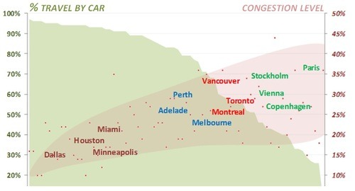
    It came from a study that looked at 74 cities in terms of two measures: the percentage of people that travel by car and the traffic congestion levels within those cities.

    The way to read the chart is to first look at the red dots. Each dot represents one of the cities studied. The position of the red dot corresponds to that city’s congestion levels. So for example, if we were to take Toronto, the congestion level is 27%.

    If you then take that same dot and draw a vertical line to the top of the green shaded area, you get the percentage of people who travel by car. In the case of Toronto, it is 56%.

    What’s interesting about this chart is that as congestion levels rise, it forces people out of their cars. In other words, the cities with the highest congestion levels also have the lowest auto share percentages.

    But the other way I interpret this chart is that the decision is almost binary: you’re either planning for cars or you’re planning for people. Based on this data, it’s hard to have both.